Interaction Nets, Combinators, and Calculus

I’ve recently posted about HVM, a highly parallel, functional runtime with awesome potential, and, just maybe, the computing model of the future.

But what what is HVM built on? From the readme we hear about things such as Interaction Nets and Lambda Calculus, but it’s hard to grasp what those are and how they relate to each-other without some investigation.

In this post, I’m going to cover some of the important concepts at a medium-high level. I’m going just deep enough to see how some of the theoretical pieces fit together, while trying to avoid getting bogged down with too many details.

Let’s get started!

Interaction Nets

The first thing to understand are Interaction Nets. Interaction Nets provide a way of programming that has some useful properties:

• They evaluate deterministically.
• They are parallel friendly, by not requiring lots of global synchronization.
• They don’t need a garbage collector to be evaluated.
• They are Turing complete, which means they can be used to represent any computation.
• They can be efficiently executed on sequential machines like our modern processors.

An interaction net is made up of an undirected graph of labeled nodes, along with a set of rules that define how nodes with different labels interact with each-other. These interactions are represented by substitutions on the graph, which move the computation forward.

Interaction Nodes

Each node in the graph must have one active port, and zero or more secondary ports. For instance, some nodes that we might use to make up a Cons list would be:

💡 Diagram Source: Some of the node examples have been taken from Yves Lafont’s paper Interaction Nets, and other examples have been taken from drawings by Victor Taelin, both were rendered into new diagrams by me.

In the diagrams, each active port is indicated with an arrow going out from a node.

Substitution Rules

Substitution rules are applied when two nodes’ active ports are connected to each-other. That’s the only time we may define substitutions. If we don’t have two active ports connected, no substitutions will happen.

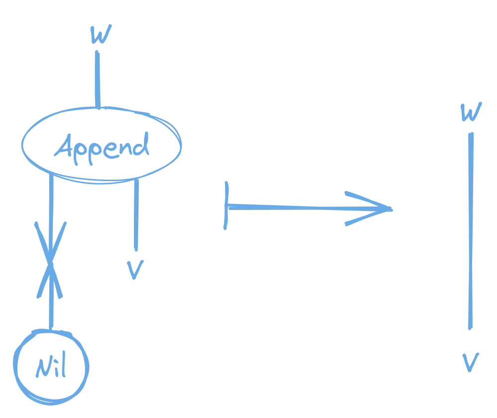
Here are the two rules we could use to implement the interaction between the Append node and the Cons and Nil nodes. This is essentially the same thing we did when we implemented List.append for HVM in my previous post.

Append to Cons Rule

Append to Nil Rule

That’s the basic idea! There are a few more restrictions and details about the concept, but I’m not going to go over them here. The restrictions make it possible to prove some of the properties of interaction nets, such as their deterministic evaluation.

Because node substitution rules are only applied on active pairs, it gives us a way to know exactly where to apply substitutions first, and we can potentially do those substitutions on different parts of the graph in parallel, which is awesome.

Symmetric Interaction Combinators

The next important concept is Symmetric Interaction Combinators. Interaction combinators are specific set of nodes and rules for interaction nets that are in fact universal. This means that any interaction net could actually be converted to an interaction net made up only of interaction combinators, and still perform the same computation.

Symmetric interaction combinators are a variant of normal interaction combinators that use the same rewrite rules for both of it’s node types, as we’ll see below.

The beauty of interaction combinators is their simplicity. There are only three kinds of nodes, and only three kinds of substitution rules.

Combinator Nodes

The three kinds of interaction combinator nodes are constructors, duplicators, and erasers.

Note: For the sake of the examples below, we don’t need to use erasers, so we’re going to leave them out for now. In concept, an eraser is a node with only one port that deletes anything that’s plugged into it, so it is easy to imagine how it might play into things after we understand constructors and duplicators.

To simplify our graphs, we’re going to display constructors and duplicators a little different than the nodes in our examples above. They will look like this:

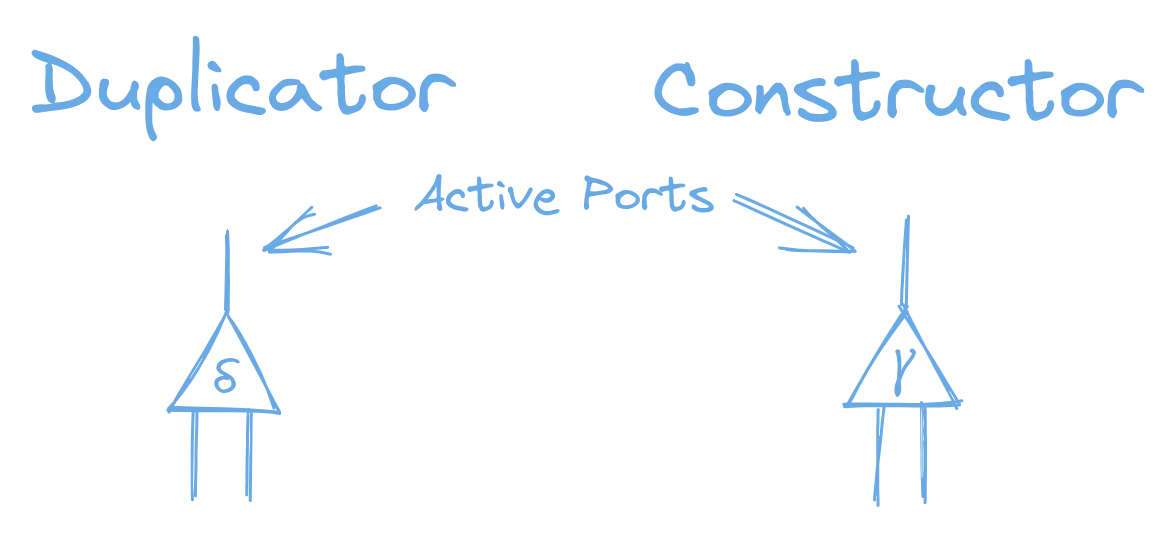
We use the greek delta symbol, δ, for duplicators, and the greek gamma symbol, γ, for constructors. Both constructors and duplicators have one active port, and two secondary ports.

Combinator Rules

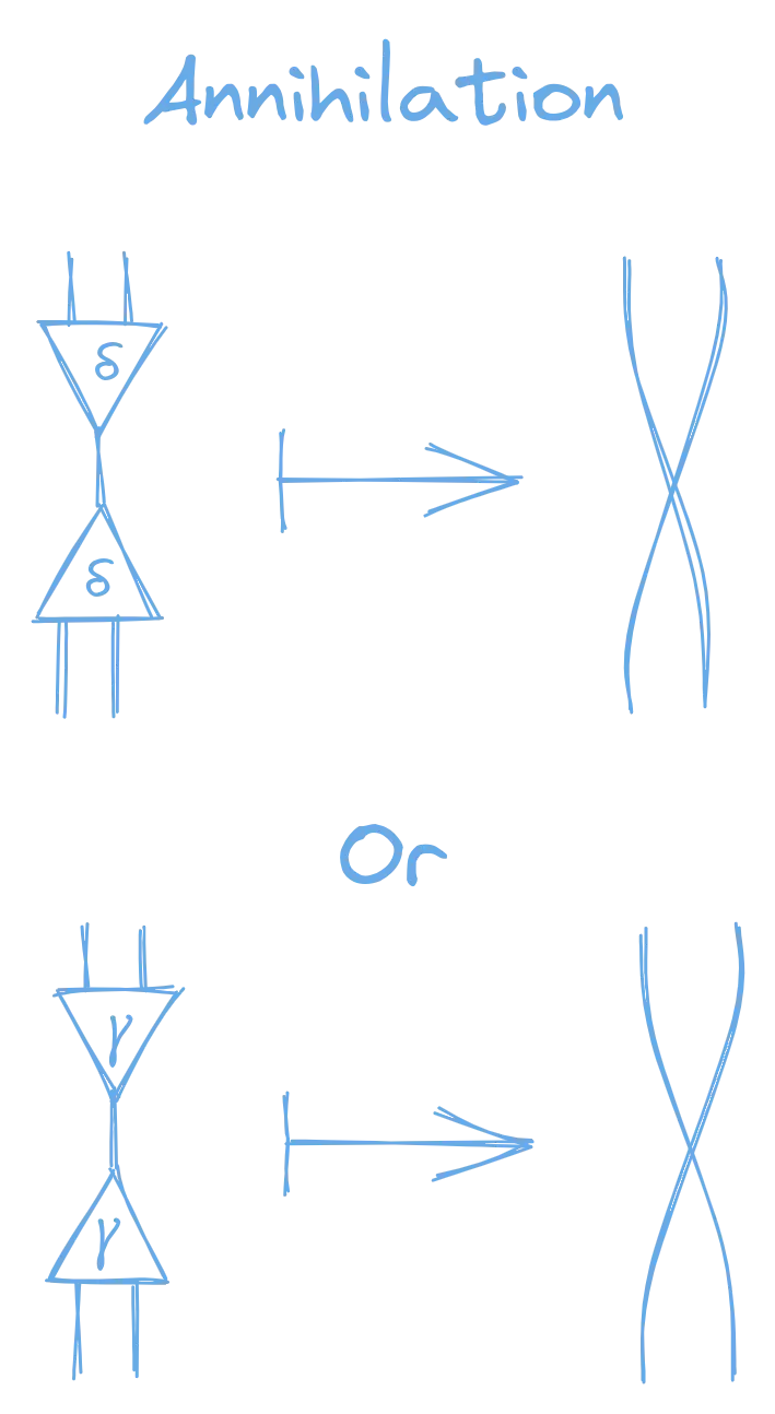
The first rule is annihilation.

Annihilation: “When the active ports of two nodes of the same kind are connected, delete the nodes, and connect their corresponding secondary ports.”

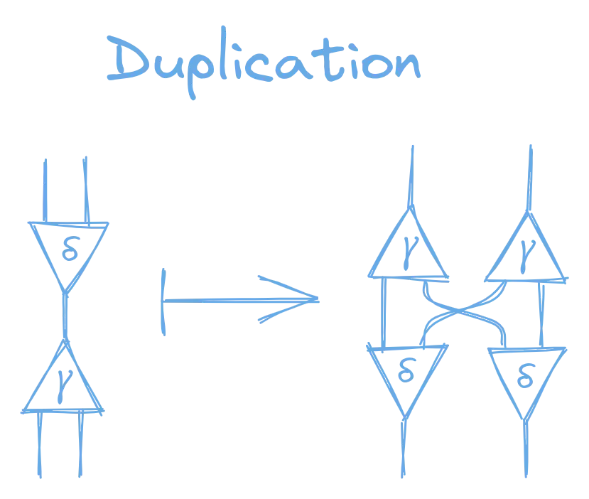
The second rule is duplication:

Duplication: “When the active ports of two nodes of different kinds are connected, then you duplicate both nodes, rotate them around, then connect the four nodes’ non-active ports to each-other.”

Combinator Computation

Computing interaction combinators happens the same way as any other interaction net:

• Search the graph for any pair of nodes with their active ports connected.
• Apply the applicable substitution for those active nodes.
• Keep repeating those steps until there are no active pairs.

Despite their simplicity, interaction combinators are still Turing complete! You can represent any computation with just constructors, duplicators, annihilations, duplications, and erasers.

But how can we go about producing interaction nets that will do the computations that we want them to? To answer that, we have to take a slight detour.

Lambda Calculus

Lambda calculus is a simple programming form that forms the foundation for functional programming, and understanding it is important to understanding how we can program with Interaction Combinators.

ℹ️ Note: LambdaExplorer.com provides a great tutorial introduction to Lambda Calculus with an interactive calculator if you want to learn more about how it works. You can even put some of the samples below into the calculator to have it reduce them.

A lambda is kind of like a function that can take a single argument, and returns it’s body.

For instance, this is a simple lambda that takes an argument, and just returns it unchanged.

λx.x;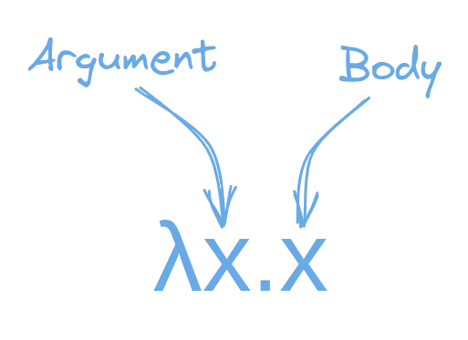

Since a lambda could return another lambda, you can use that to simulate lambdas with multiple arguments.

This lambda takes two arguments, and returns the second one unchanged.

λa.(λb.b)

Lambda Application

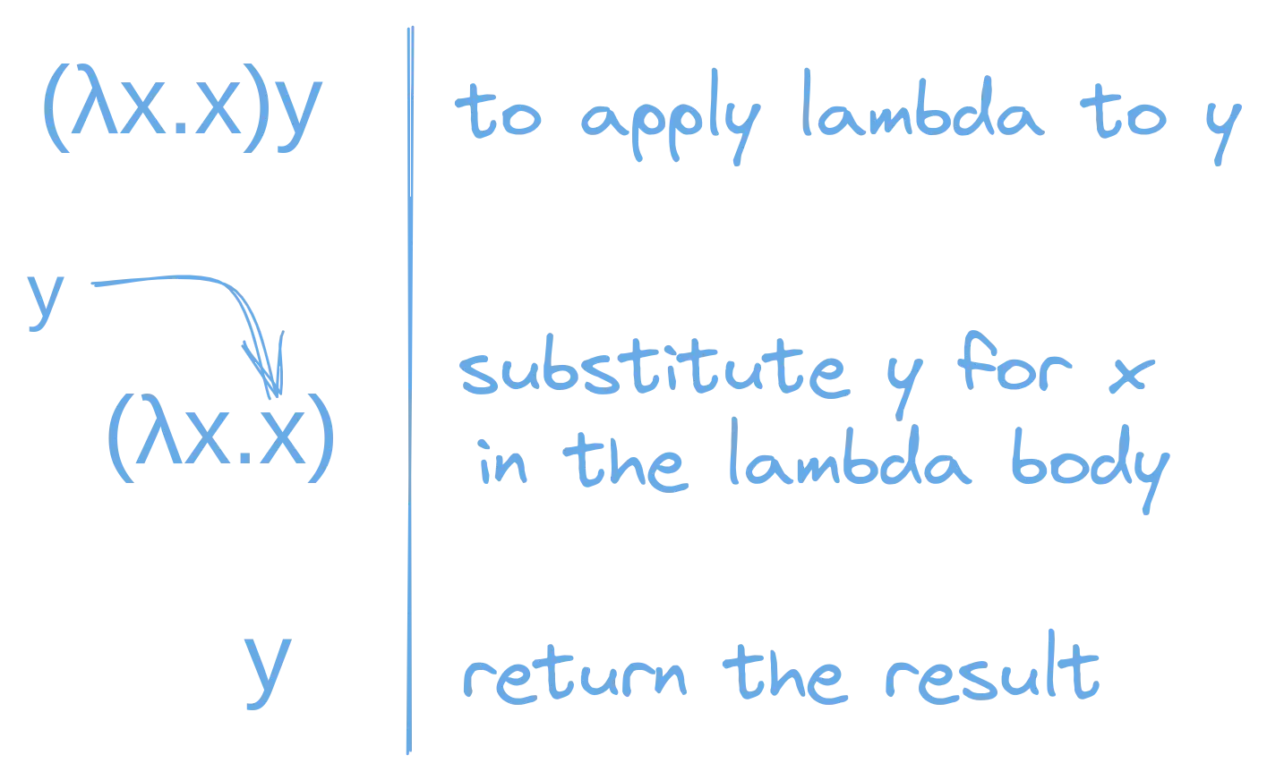
Computation is powered by Lambda Application. Lambda application is kind of like calling the lambda like a function. You take the lambda body and substitute all occurrences of the lambda’s argument for some value.

We indicate lambda application by placing one expression after another. So xy actually means, “Apply x to y”.

For example, if we apply (λx.x) to the variable y we get.

For another example, here is a lambda that means: “take an argument x and then apply x to itself”:

λx.xx;

Once there are no more lambda applications to make, we have reached what we call the normal form, and the computation is done.

Let’s look at one more lambda expression and see how it reduces to normal form:

λx.xx(λx.x)(
  // Replace each `x` in the first lambda's body with (λx.x)
  λx.x
)(λx.x); // Again, replace the `x` in the first lambda's body with (λx.x)
λx.x;

If this doesn’t make sense to you yet, maybe go through the lambda explorer tutorial to get a better idea of what’s going on. It’s got a really great walk-through.

Interaction Calculus

Finally we introduce Interaction Calculus. Interaction Calculus is a language inspired by lambda calculus, that, in fact, represents a net of interaction combinators.

We can quite simply represent lambdas and lambda applications with interaction combinator constructor nodes, and we can use a duplicator node whenever we need to use a value twice. We also introduce the root node, which represents the end result of the computation.

The “Function” and “Output” ports deserve a little bit more explanation.

• If a Lambda node’s Output port is connected to the Root, that indicates that the result of the computation is a lambda.
• If a Lambda node’s Output port is connected to the Function port of an Application node, then that indicates lambda application.

Note that you may still connect the Function port of application nodes to different kinds of ports, other than a Lambda Output port. This could happen, for instance, if the return value of another lambda application is also lambda, and you wish to make a lambda application on that returned lambda.

Example Expressions

For instance, if we want to represent the simple lambda λx.x, which just returns it’s argument, we would do that with an interaction net like this:

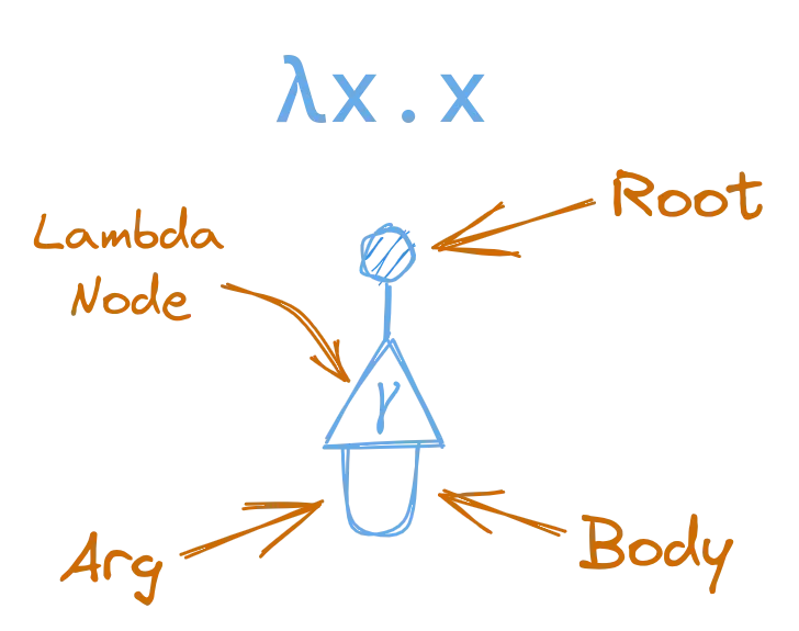
Notice how the argument port of the lambda, is connected to the body port of the lambda in a loop, as representative of the lambda taking it’s argument, and using it as it’s body.

Here’s another example for λx.xx.

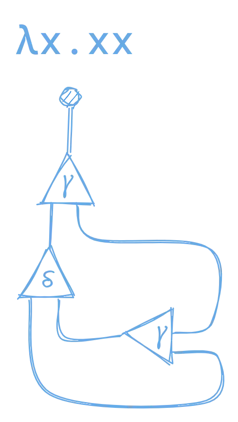
This is a lot more complicated, so let’s try to break it down. We can see that this expression is made up of one lambda node, one duplicator node, and one lambda application node.

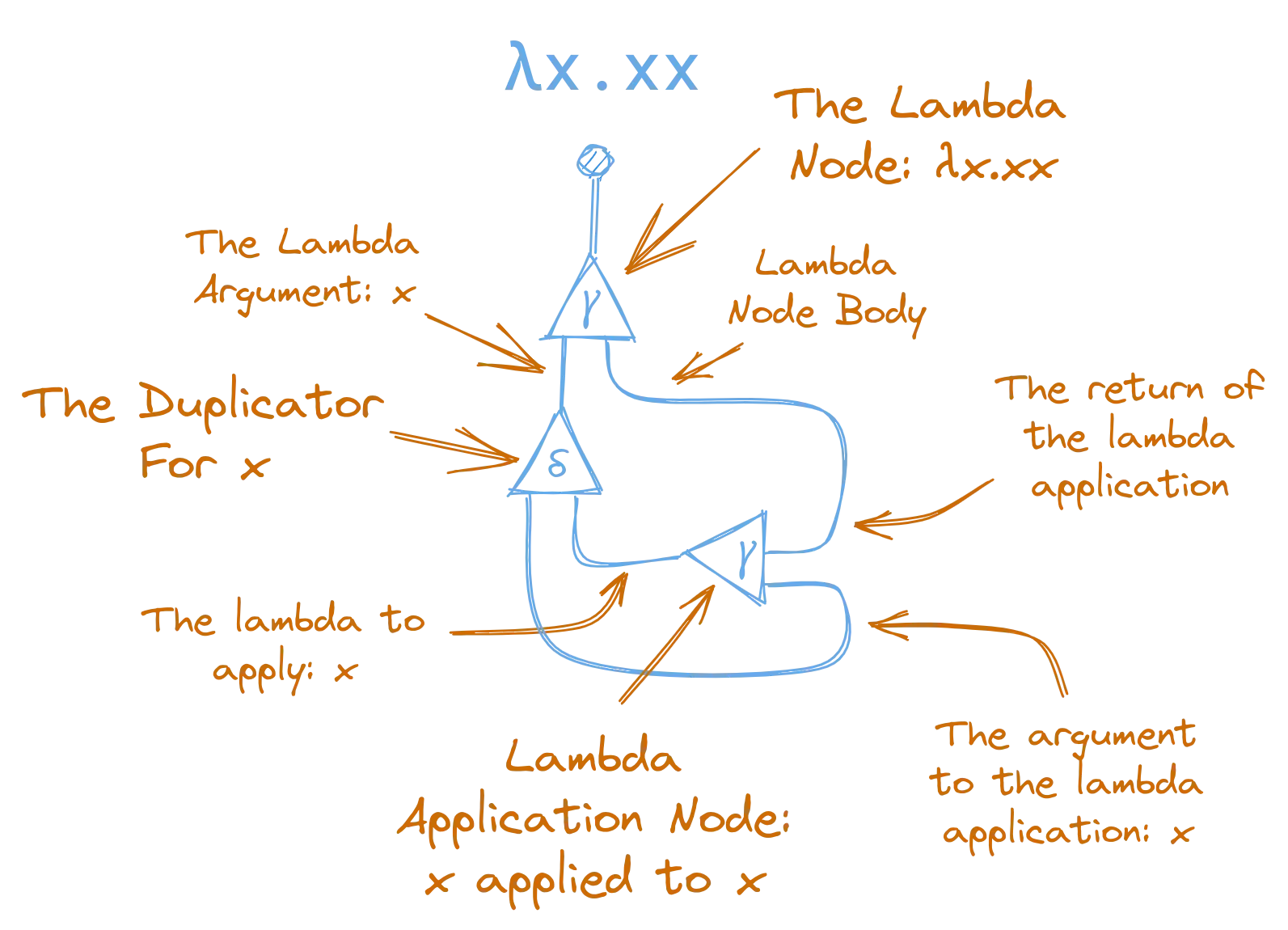
If you follow it slowly you can see how this net does exactly what lambda expression does: it is a lambda, where the argument is taken, duplicated, and then applied to itself, before being returned as the body of the lambda.

If you don’t get it right away, don’t worry, it’s a little tricky! Just try to follow the process carefully and compare the node ports and connections with the list of nodes above.

A Reducible Expression

Once you’ve got that down, lets see what (λx.xx)(λx.x) looks like. Note that the previous examples were already in their normal form, but this expression is not. Again, if you look carefully at the above two graphs, neither of them had any active pairs, so there are no substitutions that we could make.

But, if we represent (λx.xx)(λx.x) as a graph, it is not in normal form, and will therefore have active pairs that we can reduce.

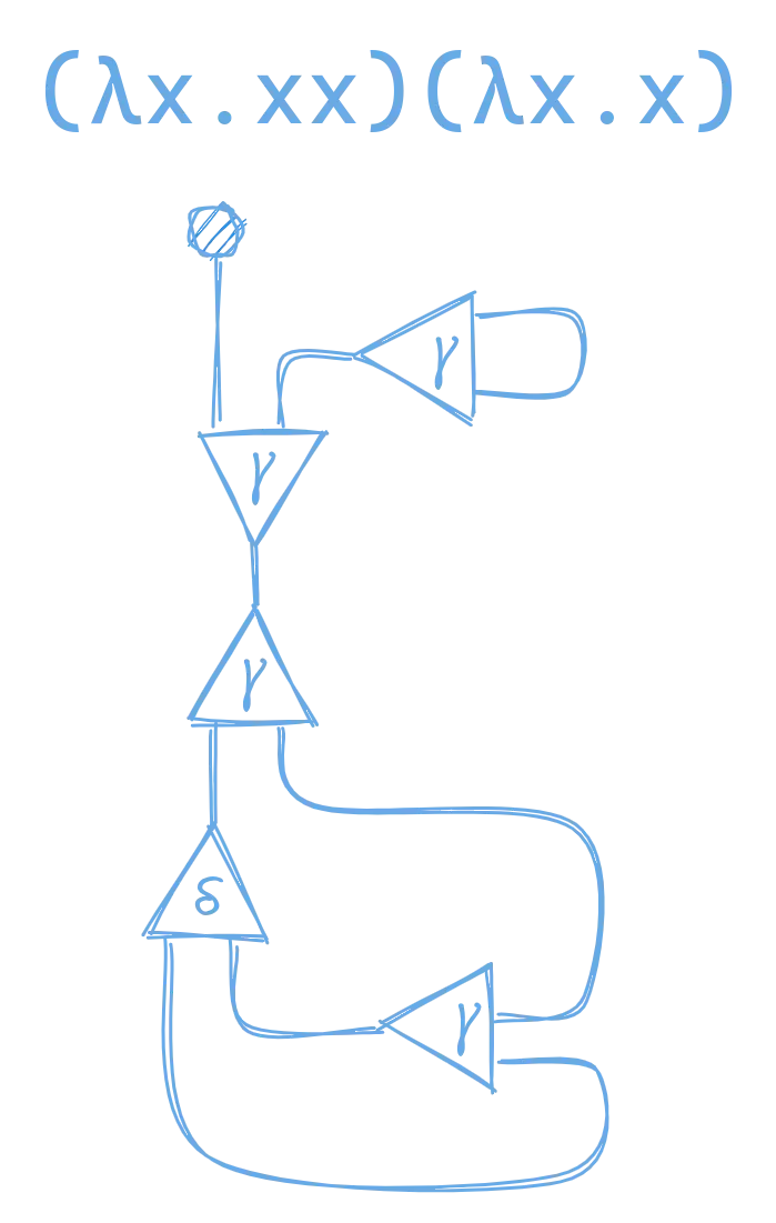
If you break this down you can see it’s made by combining our graphs for (λx.xx) and (λx.x) with a lambda application node:

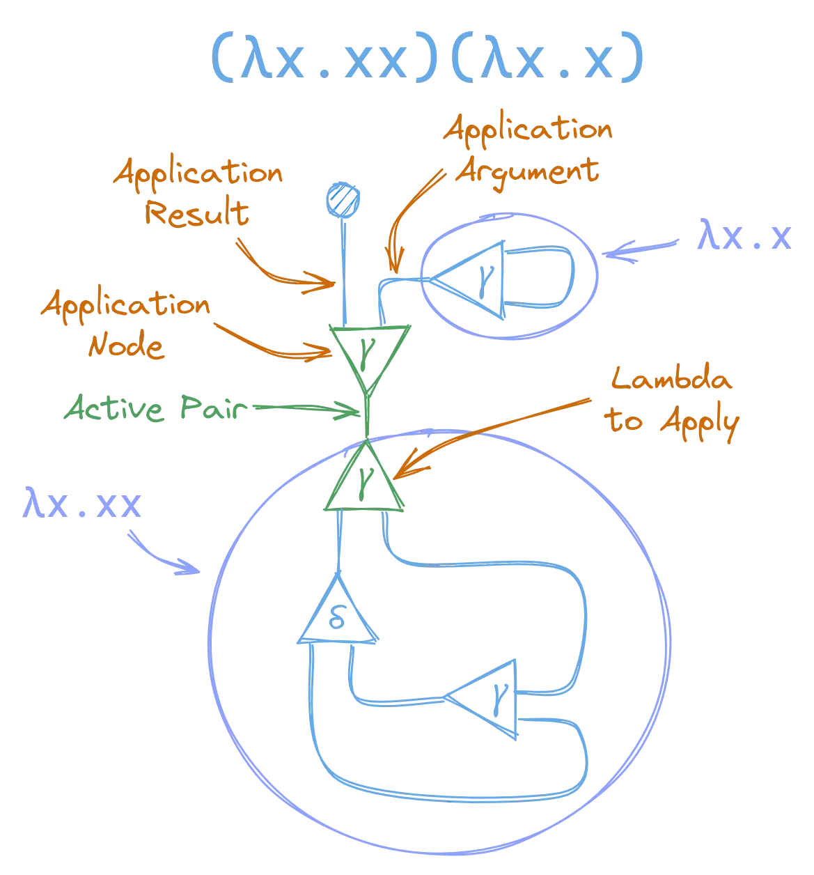
Now that we have an active pair, between two nodes of the same kind, we can apply our annihilation rule, and begin reducing the graph to normal form. This gives us a new graph:

And now there’s a new active pair, so we can further reduce this graph. This time the active pair contains a constructor and a duplicator node, so we need to use the duplication rule.

This also created another active pair, so we apply the annihilation rule again, and finally, one more time.

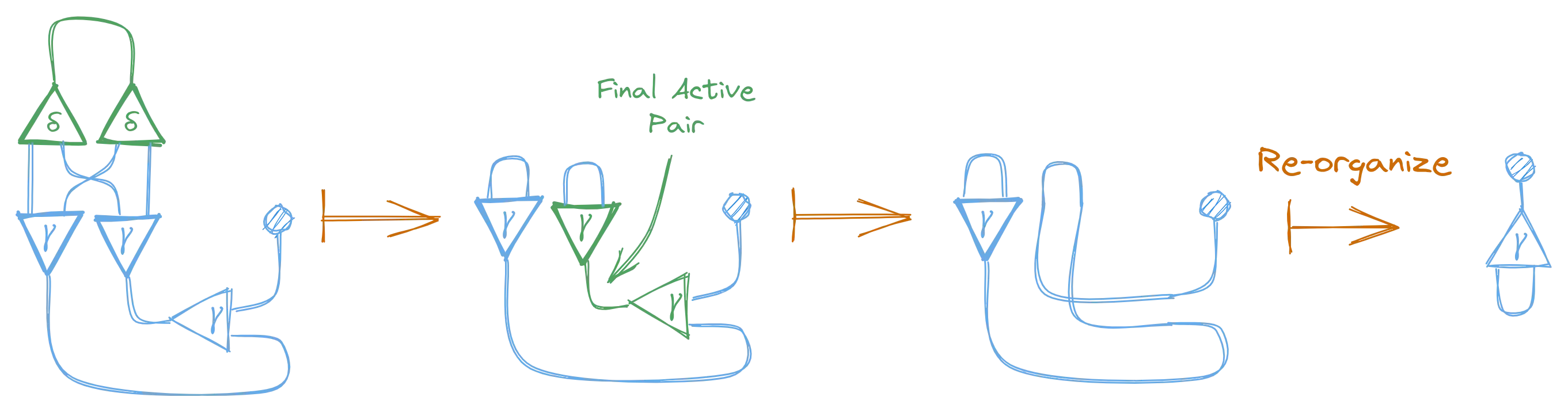
And look at that, the final graph is the same as the graph for λx.x, which, in fact, is the normal form of (λx.xx)(λx.x)! We just reduced a lambda expression using interaction combinators!

An amazing thing about reducing lambda expressions like this is that the reductions are optimal, meaning that they avoid unnecessary work.

Relation to Lambda Calculus

A caveat of this technique for reducing lambdas is that it doesn’t exactly match the behavior of the normal lambda calculus. While it might reduce the same as the normal lambda calculus in many cases, it doesn’t always. And that’s totally fine, it doesn’t need to match perfectly to be useful in it’s own right.

Another thing to be aware of is that certain terms that can reduce under lambda calculus don’t reduce under interaction calculus, but this is a rare edge-case.

I also haven’t covered the whole set of rules for interaction calculus here. You can read a little more by checking the comments in the source code for the latest implementation of interaction calculus in the Kind language.

Relation to Garbage Collection

Part of the key to HVMs performance is the way that it doesn’t need a garbage collector, and that is partially owed to the semantics of interaction calculus. It just so happens that the interaction between constructor and duplicator nodes gives us a way to incrementally clone a lambda expression. This is incredibly important to being able to avoid using references and keep things simple and performant.

You can read a bit more about this in the What Makes it Fast section of the work-in-progress HVM explanation doc.

Summary

And that concludes your tour! We’ve taken an ultra quick look at a lot of the foundational theoretical elements behind HVM and, while some of it’s a little hard to wrap your head around, it’s also not that complicated!

It’s really exciting to me that such a powerful concept can be expressed in such simple terms, and I’m intrigued enough that I might play around with my own implementation just to see how simple it could be to make a runtime that out-performs runtimes like Python, JavaScript, etc.

I just started investigating all of this 4 days ago, so my understanding on any of these topics may not be 100% accurate. If somebody find somethings incorrect in this post, I’d be grateful if you opened a discussion so that I can correct it.

I can’t wait to keep learning and trying stuff out. I’ll be posting more as I progress. To the future! 🚀

Appendix: After I wrote this, one reader noticed that I didn’t do proper justice to the eraser node. They went on a journey of their own, figuring out how to represent 0 + 1 with interaction nets. If you want to follow along check out @stevenhuyn’s great follow up post. Thanks for continuing the investigation @stevenhuyn!